Project 4

CS180 - Fall 2024 Alex Cao

Introduction

In this project, I will start by trying to find homographies between images. These homographies are essential for understanding the geometric relationships between different views of a scene. Then, using these homographies, I will warp images to perform rectification and image stitching. Rectification will make the images appear rectified, while stitching will combine them into a seamless panorama. This process involves complex mathematical transformations and computer vision techniques to create a cohesive final image from multiple input photographs.

Part 1: Pictures

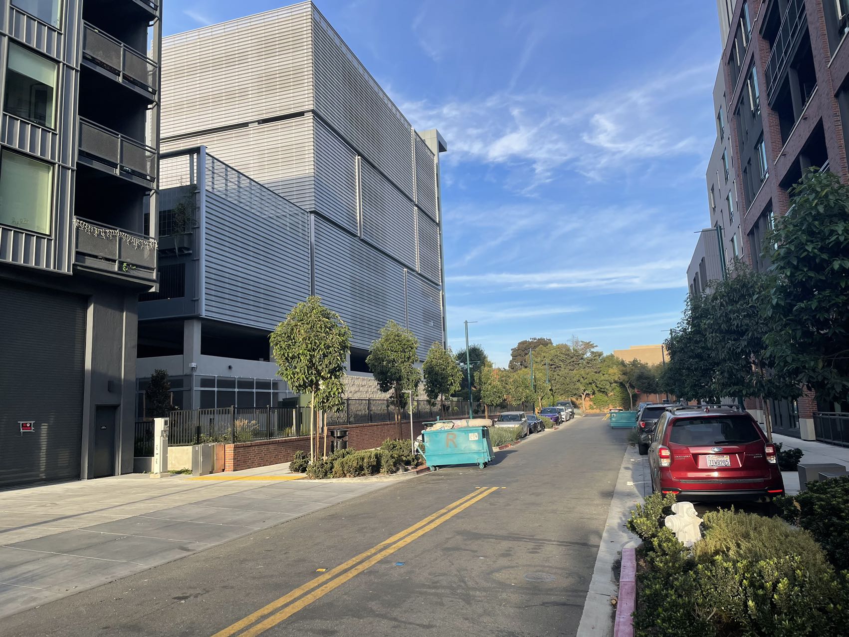
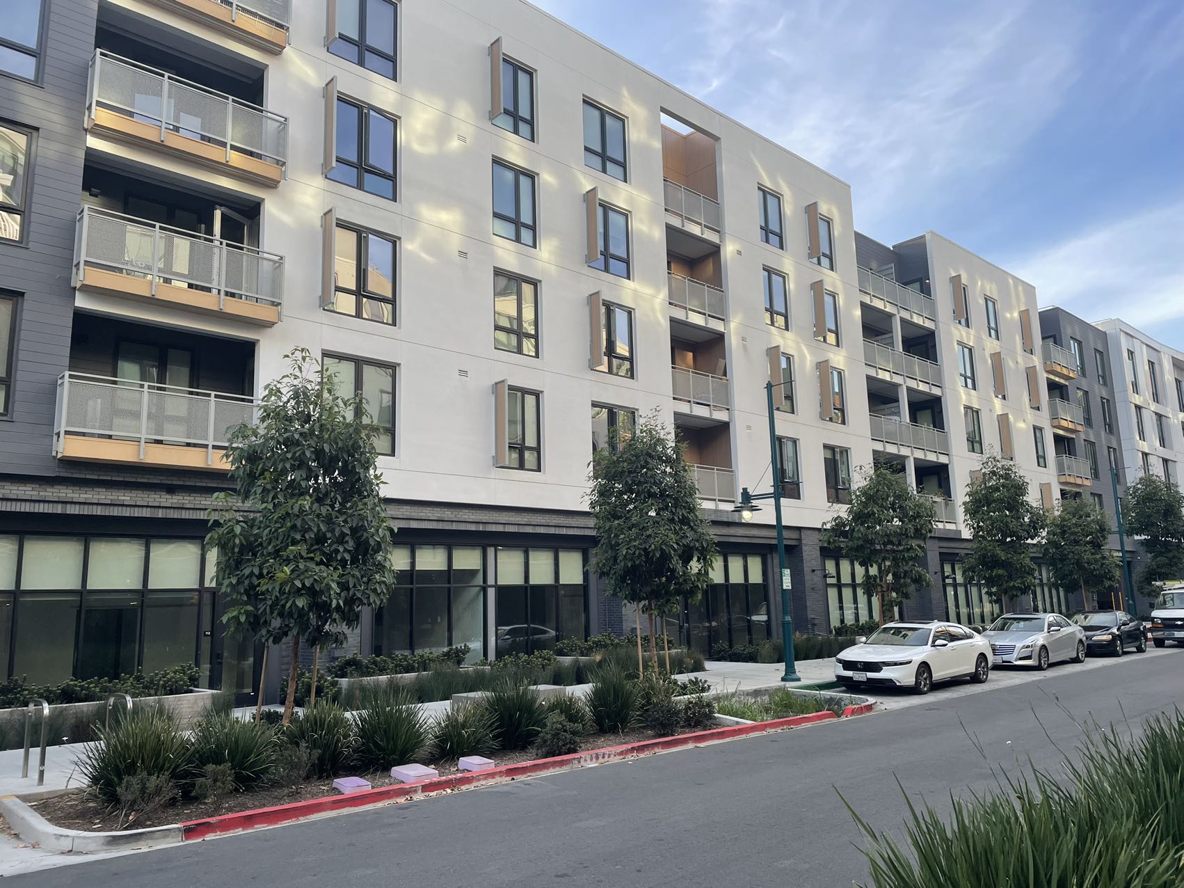
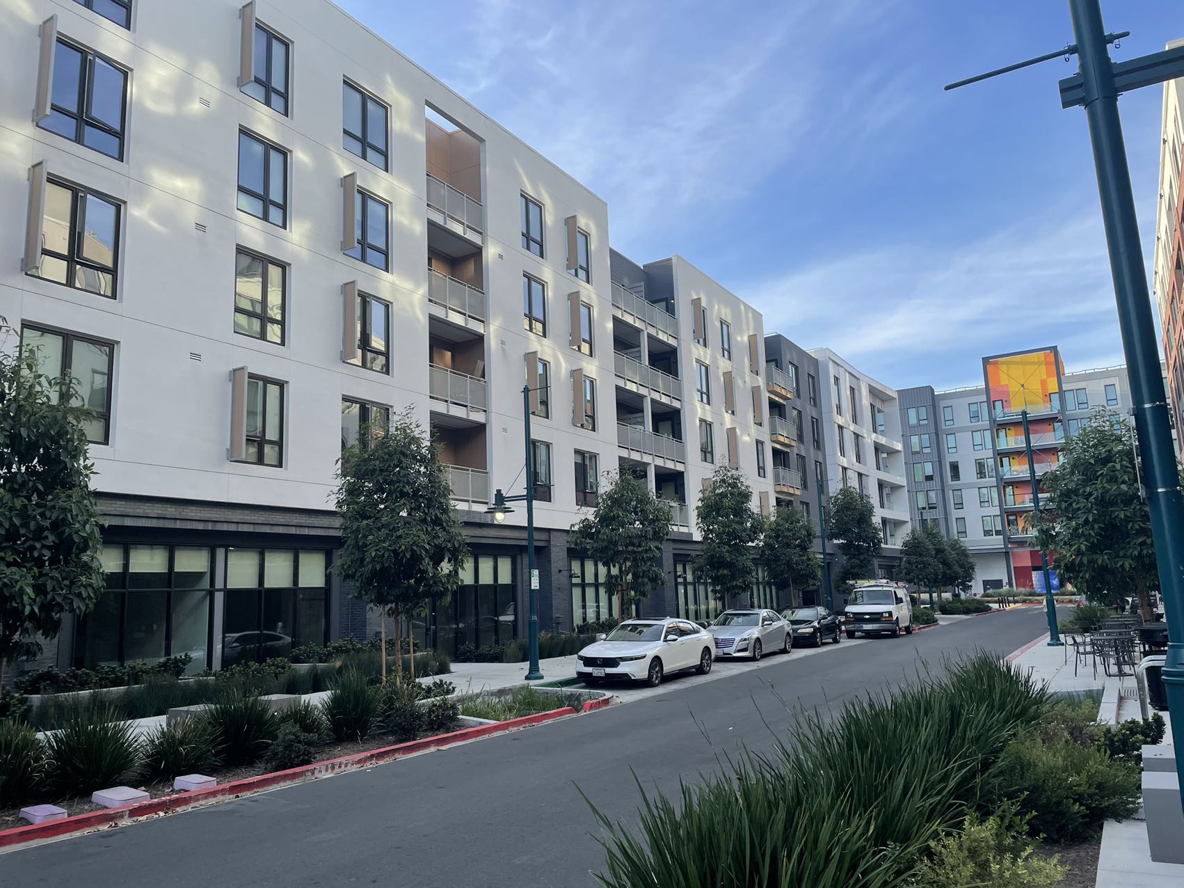
In this part, I took several set of pictures from a single center of projection.

Image 1

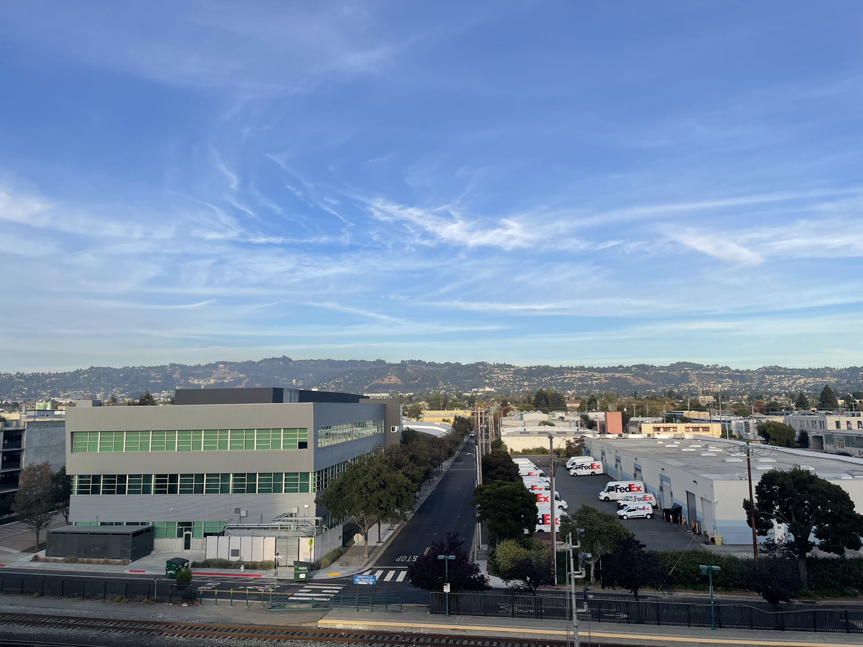
Image of balcony view captured from the left angle.

Image 2

Image of balcony view captured from the right angle.

Image 1

Image of garage captured from the left angle.

Image 2

Image of garage captured from the right angle.

Image 1

Image of downstairs the Emery apartment captured from the left angle.

Image 2

Image of upstairs the Emery apartment captured from the right angle.

Part 2: Recover Homographies

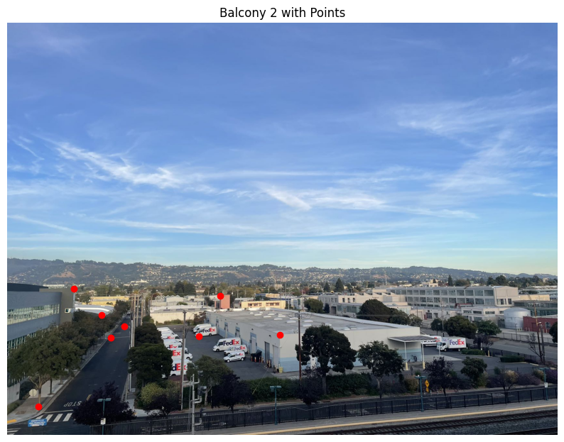
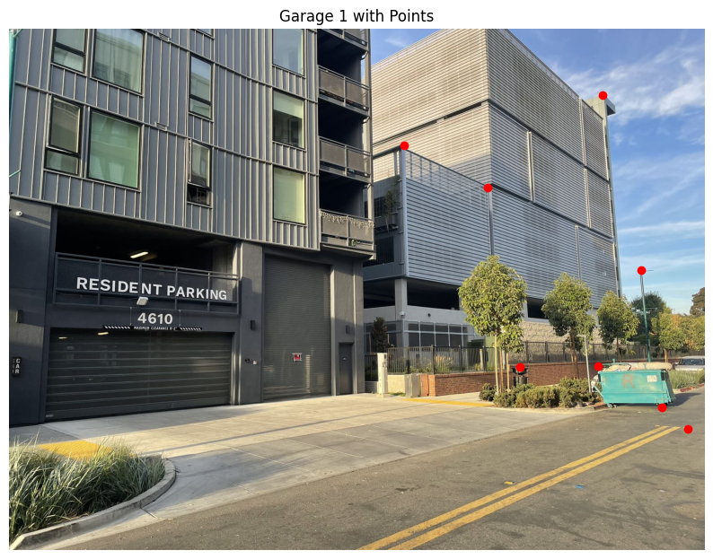
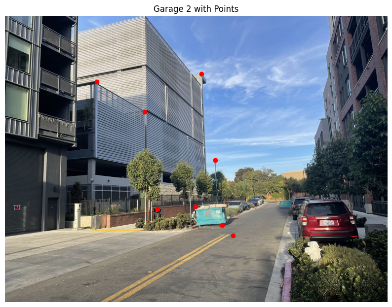
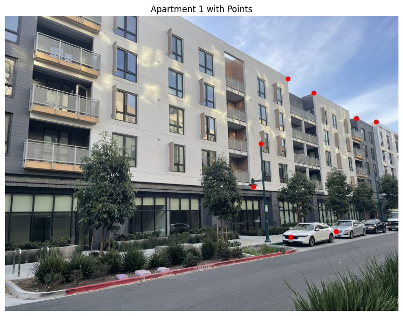
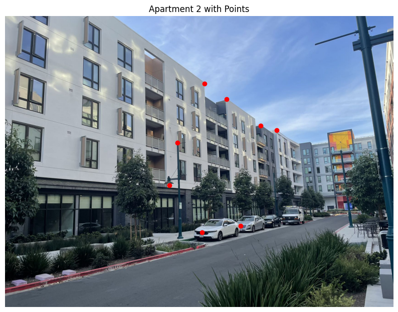
The first step is to find Homographies transform between images. To find the transformation matrix, first we need to lable the correspondence points between images. In this project, I used this online tool to label the points.

Homography Image 1

Point correspondences

Homography Image 2

Point correspondences

Homography Image 1

Point correspondences

Homography Image 2

Point correspondences

Homography Image 1

Point correspondences

Homography Image 2

Point correspondences

To find the homography matrix, we can set up the following equation: (adapted from the slides)

\[ \begin{bmatrix} a & b & c \\ d & e & f \\ g & h & 1 \end{bmatrix} \begin{bmatrix} x \\ y \\ 1 \end{bmatrix} = \begin{bmatrix} wx' \\ wy' \\ w \end{bmatrix} \]

To solve this, we can expand the terms, and that would be:

\[ \begin{align*} &\begin{cases} ax + by + c = wx' \\ dx + ey + f = wy' \\ gx + hy + 1 = w \end{cases} \\[10pt] \implies &\begin{cases} ax + by + c = (gx + hy + 1) x' \\ dx + ey + f = (gx + hy + 1) y' \end{cases} \\[10pt] \implies &\begin{cases} ax + by + c - gxx' - hyx' = x' \\ dx + ey + f - gxy' - hyy' = y' \end{cases} \\[10pt] \implies &\begin{bmatrix} x & y & 1 & 0 & 0 & 0 & -xx' & -yx' \\ 0 & 0 & 0 & x & y & 1 & -xy' & -yy' \end{bmatrix} \begin{bmatrix} a \\ b \\ c \\ d \\ e \\ f \\ g \\ h \end{bmatrix} = \begin{bmatrix} x' \\ y' \end{bmatrix} \end{align*} \]

We can then use least square to solve for the homography matrix.

Part 3: Image Warping

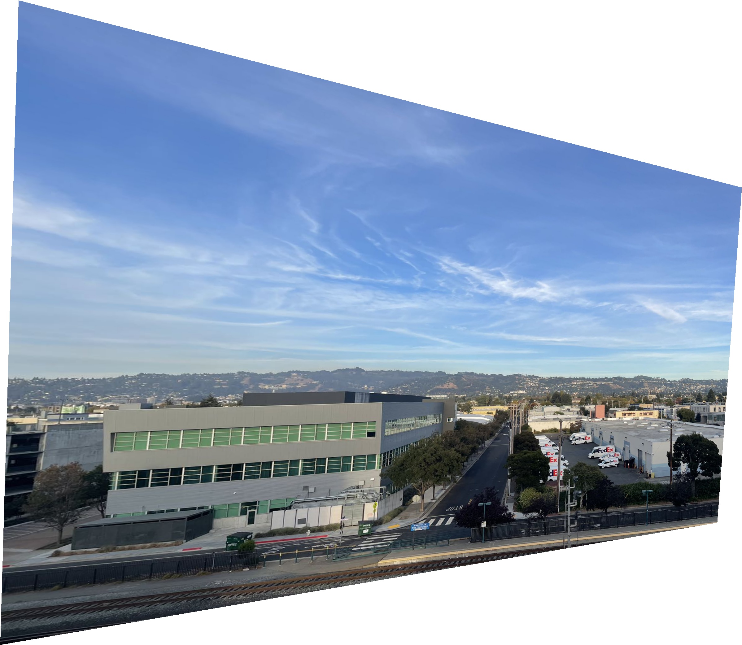
Once we have the homography matrix, we can use it to warp the images to a different space. This can be done using the inverse warping from last project. Specifically, once we have the homography matrix, we can first determine the output shape by transforming the corner points of the image. After we have the output shape, we can do inverse warping and fill in the values from the original image using bilinear interpolation. Below is one result of warping the balcony left view into the same space as the balcony right view.

Warp Image 1

Original balcony left view before warping.

Warp Image 2

Warped balcony left view into the same space as the balcony right view.

Part 4: Image Rectification

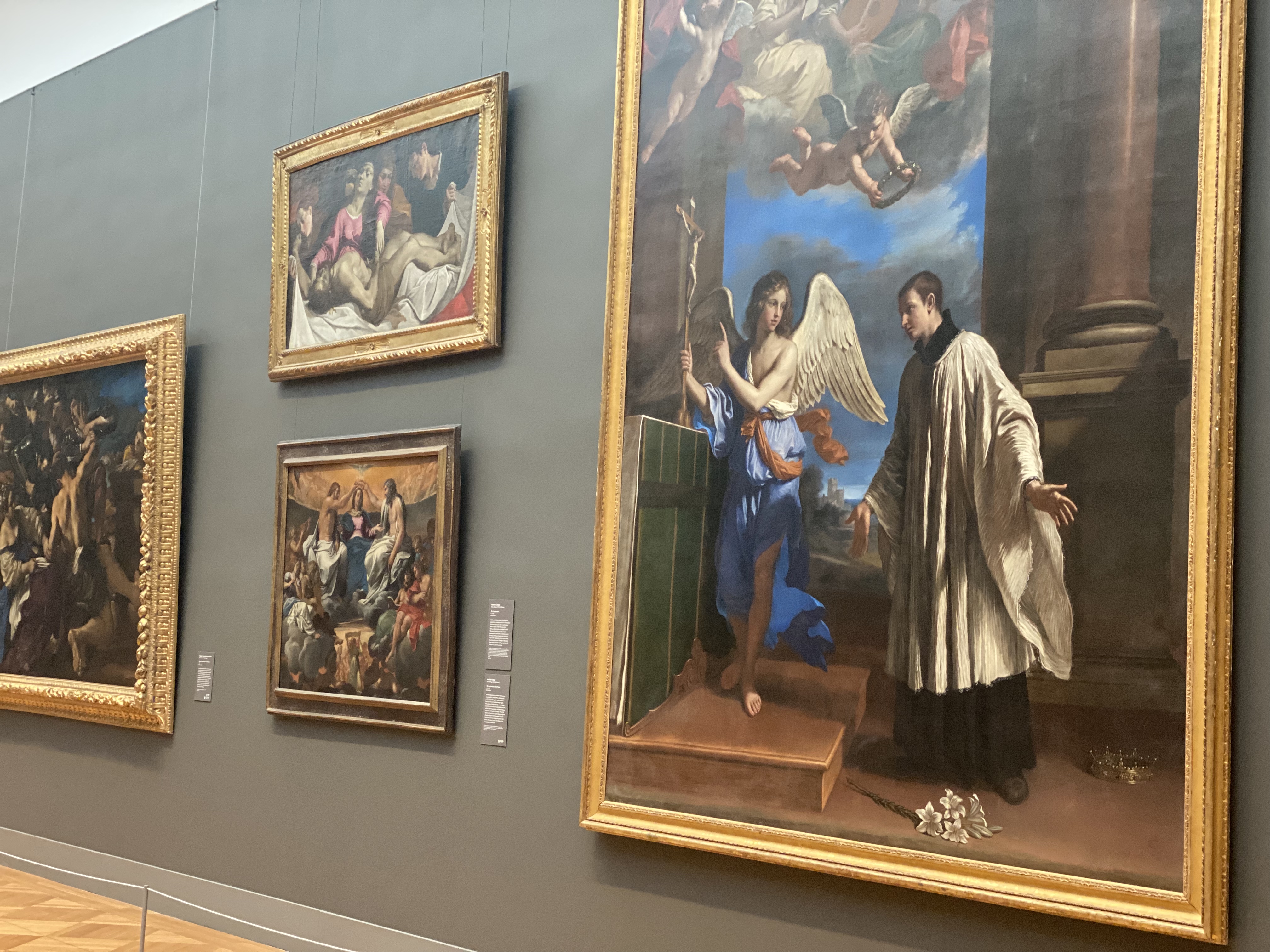
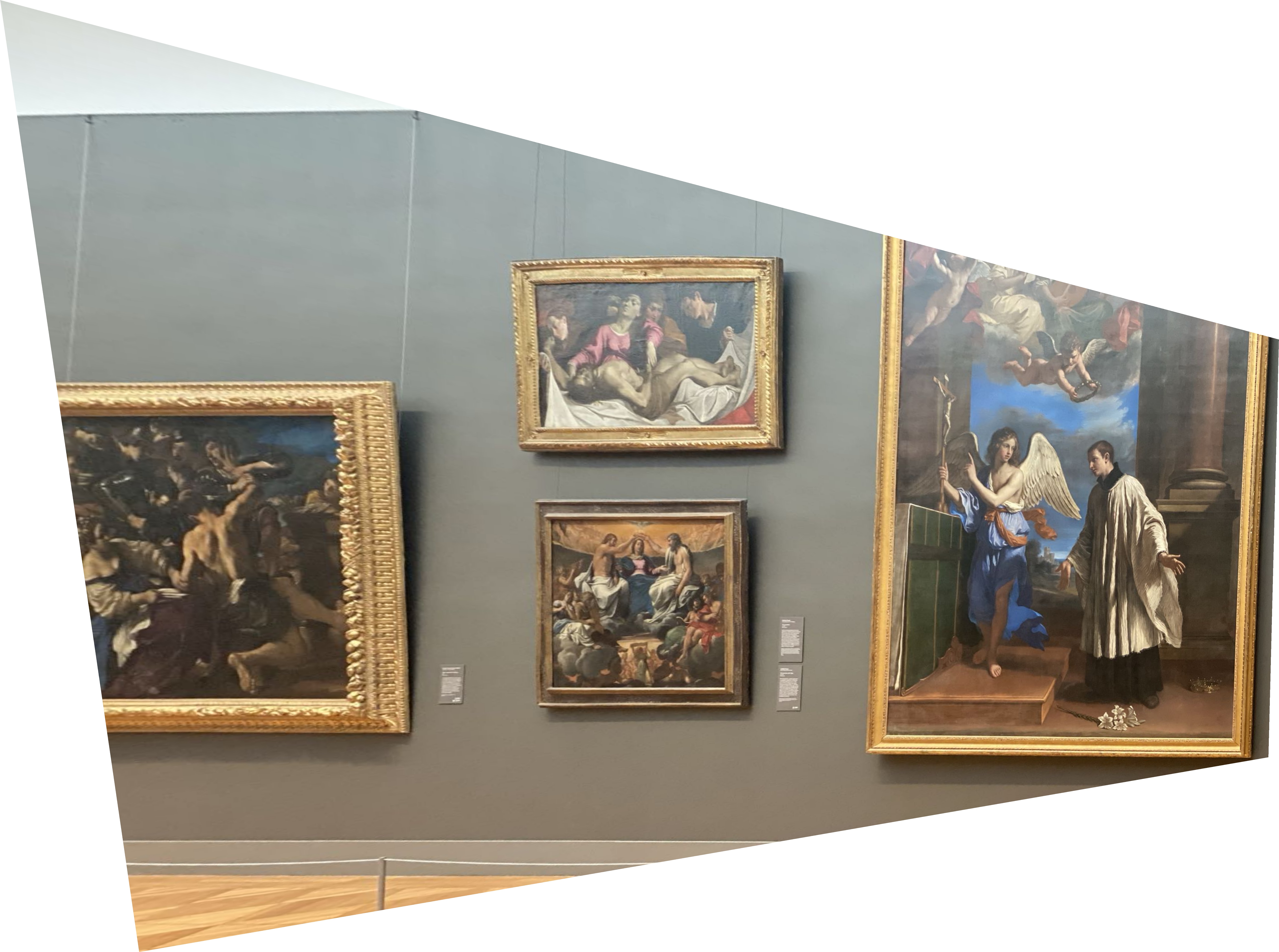
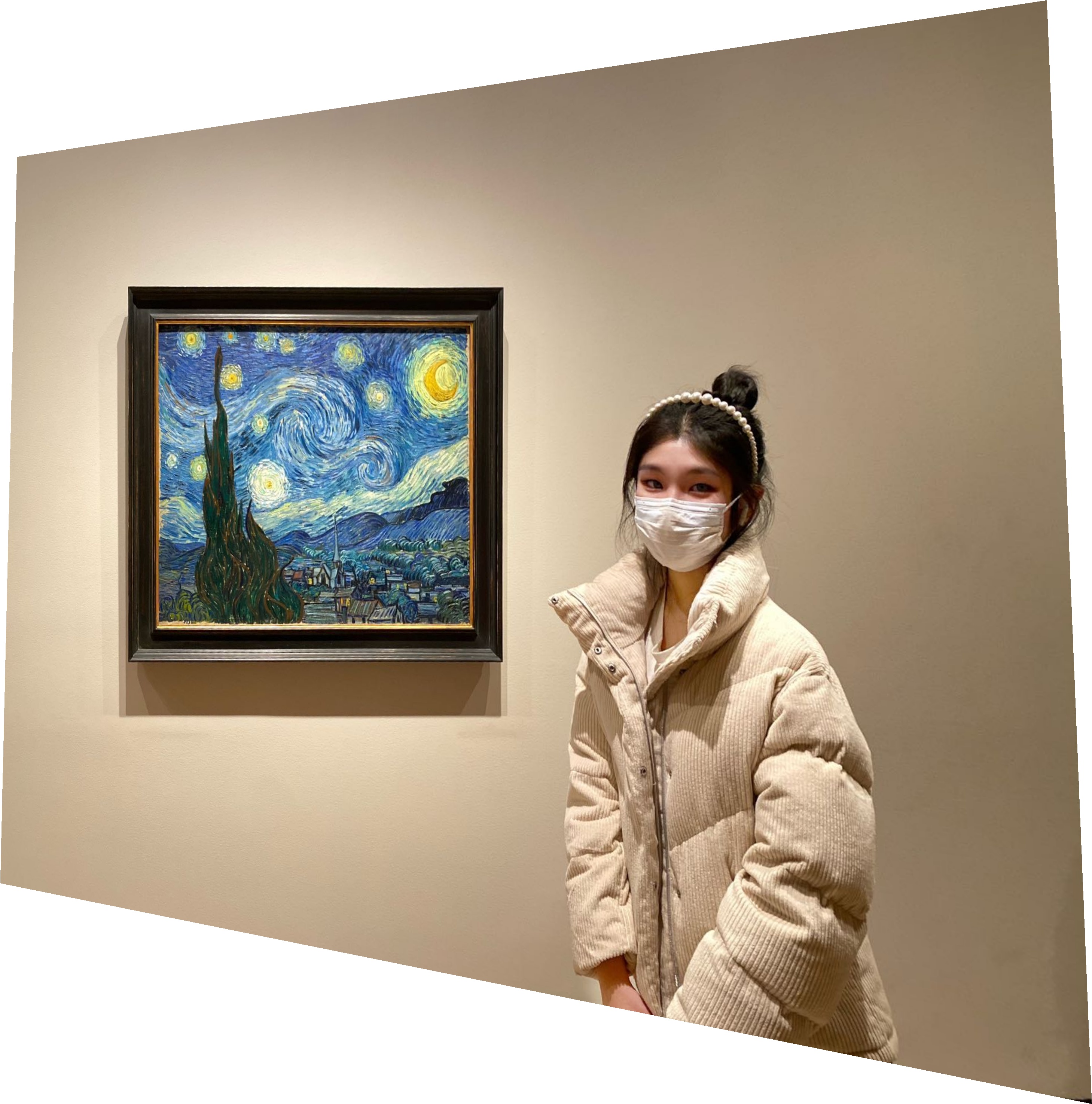
One fun thing we can do with homography is image rectification, where we can warp the images to some space so that it appears that we are looking directly from above. If we know something would look like a square when we are directly staring it, we can create a square ourself and warp the image into that square using homography. Below is an example of rectifying a picture of a painting.

Blend Image 1

Before rectification.

Blend Image 2

After rectification.

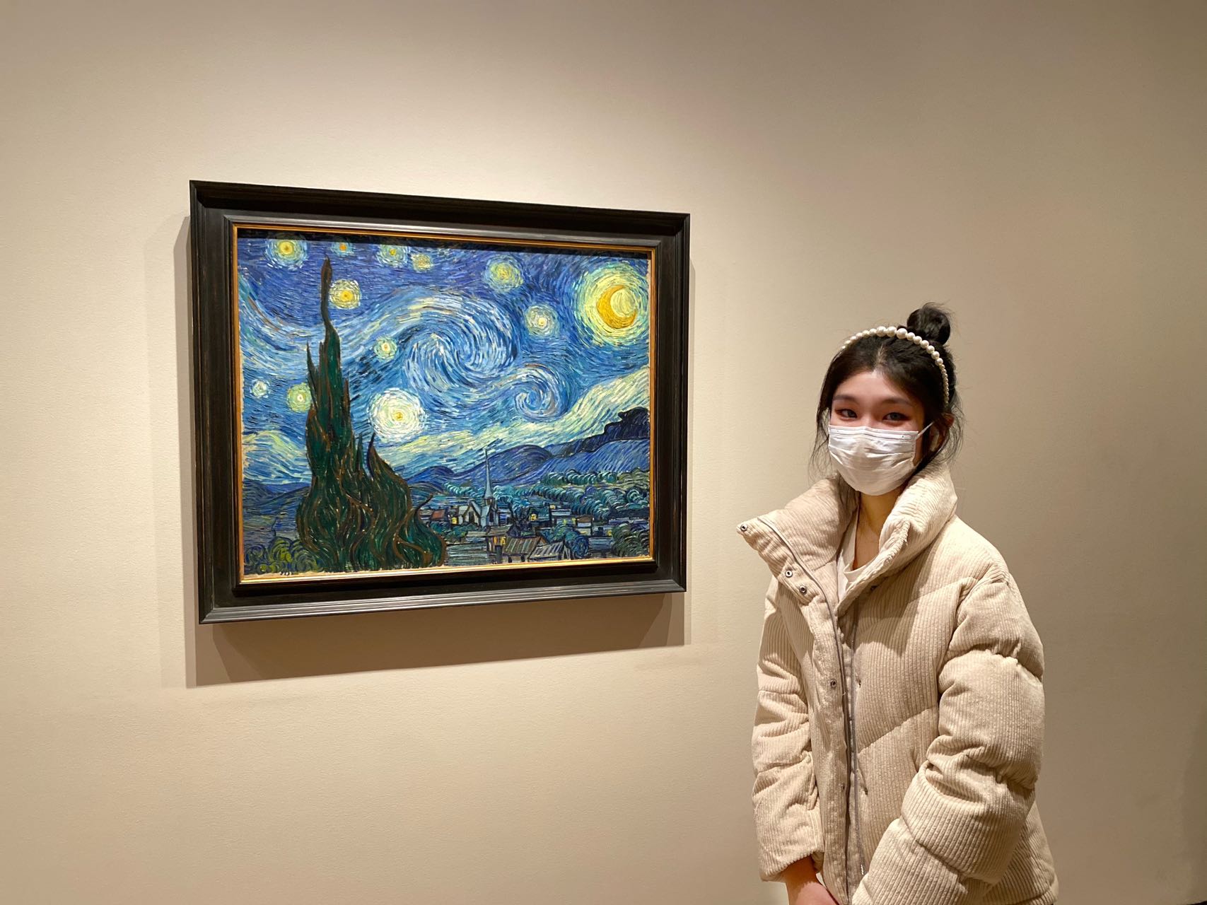
Here is another example, where a Van Gogh painting is rectified to a square. (It would be better warp this into a rectangle, but I am purposely making it a square to show how it would look in a square.)

Blend Image 1

Before rectification.

Blend Image 2

After rectification.

Part 5: Image Stitching

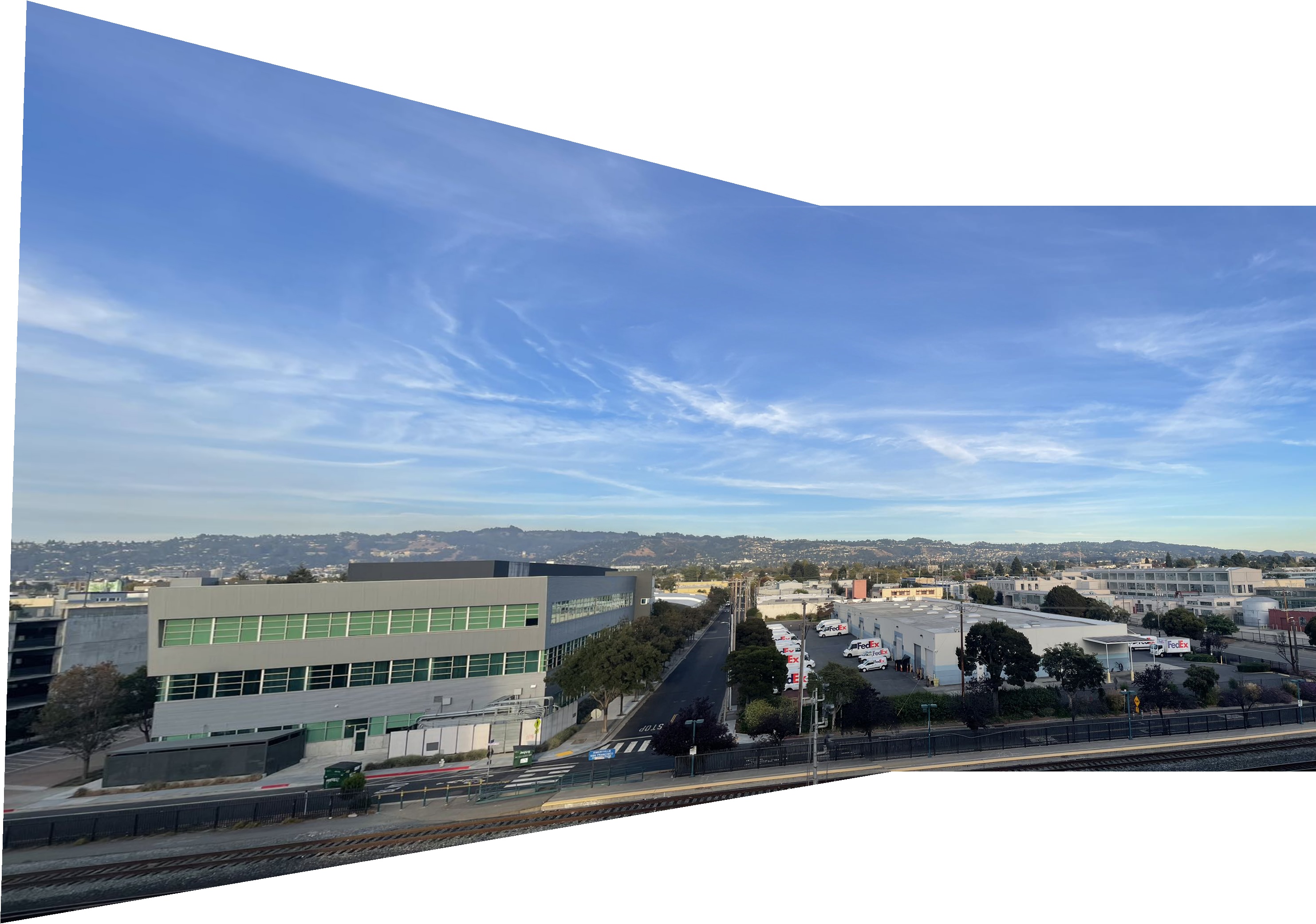
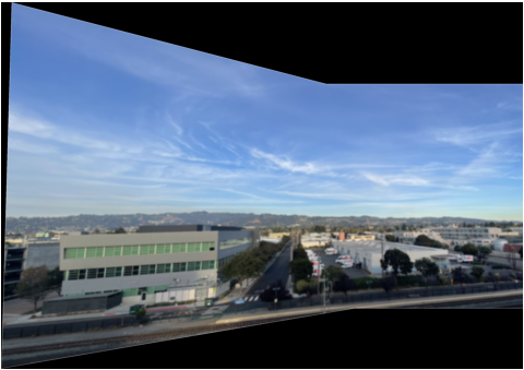
Another fun thing homography can achieve is image stiching. When two pictures are taken from the same center of projection, we can use homography to transform the first image to the space of second image. To align the images, we first calculate the shift between image1 undergoes after homography transformation. Then, we apply the same shift to image2 to align the images. Note that the alignment is not perfect, because we calculated our homography transformation using least square, but this error is minor and not noticeable in stiching.

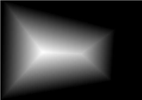
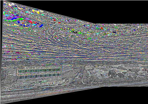
Simply aligning the image is not enough for a good stiching. We also need a way to smooth out the region where the images overlap. If we naively take the average of the two images, we can see a very clear edge at the overlap region. To fix this, I will be using two band blending, where I first calculate the L2 distance transform of the alpha masks (which pixels are used in the final result), I then use the normalized distance transform of two pictures to perform blending. Specifically, I first find the high frequency and low frequency components of the two images. For high frequency, the pixel where it's distance transform value is greater will be taken between the two images. For low frequency, the distance transform serves as weights for a weighted average of the two images.
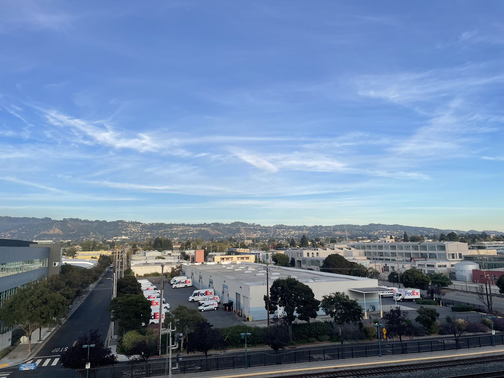
Final Mosaic 1

balcony left image

Final Mosaic 2

balcony right image

Final Mosaic 1

L2 distance transform of the alpha mask of the balcony left image.
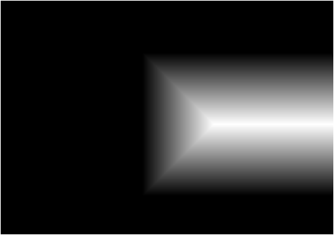
Final Mosaic 2

L2 distance transform of the alpha mask of the balcony right image.
Final Mosaic 1

low band blending

Final Mosaic 2

high band blending

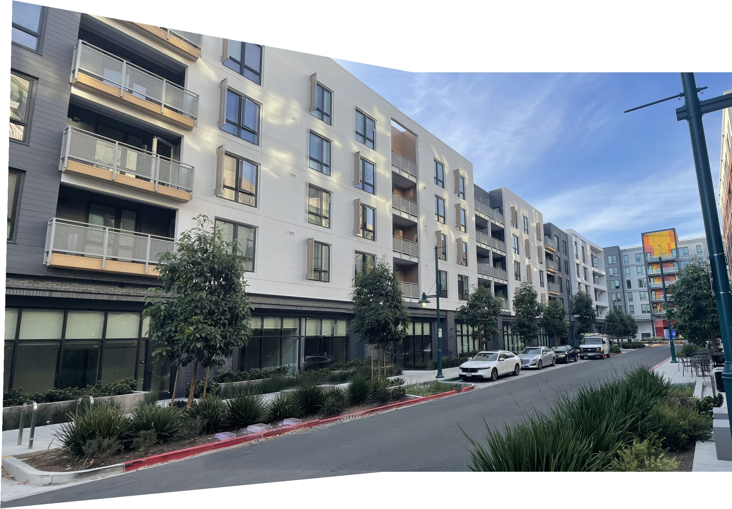
Stitched Balcony Image

Final stitched balcony image

Here are a few more examples, the distance transform and 2 band results are not shown for simplicity of the webpage.
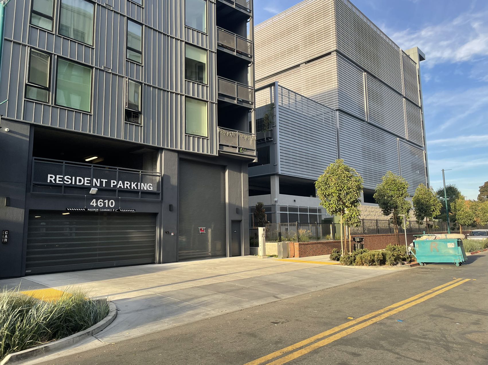
Final Mosaic 1

garage left image

Final Mosaic 2

garage right image

Stitched Balcony Image

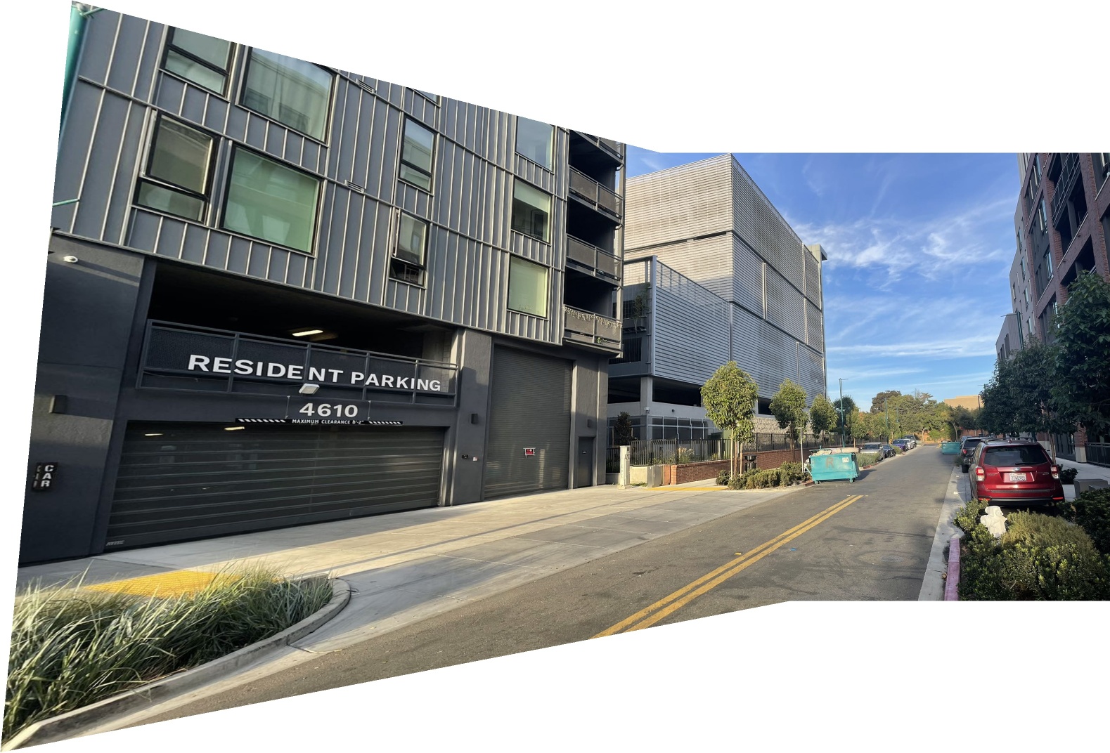
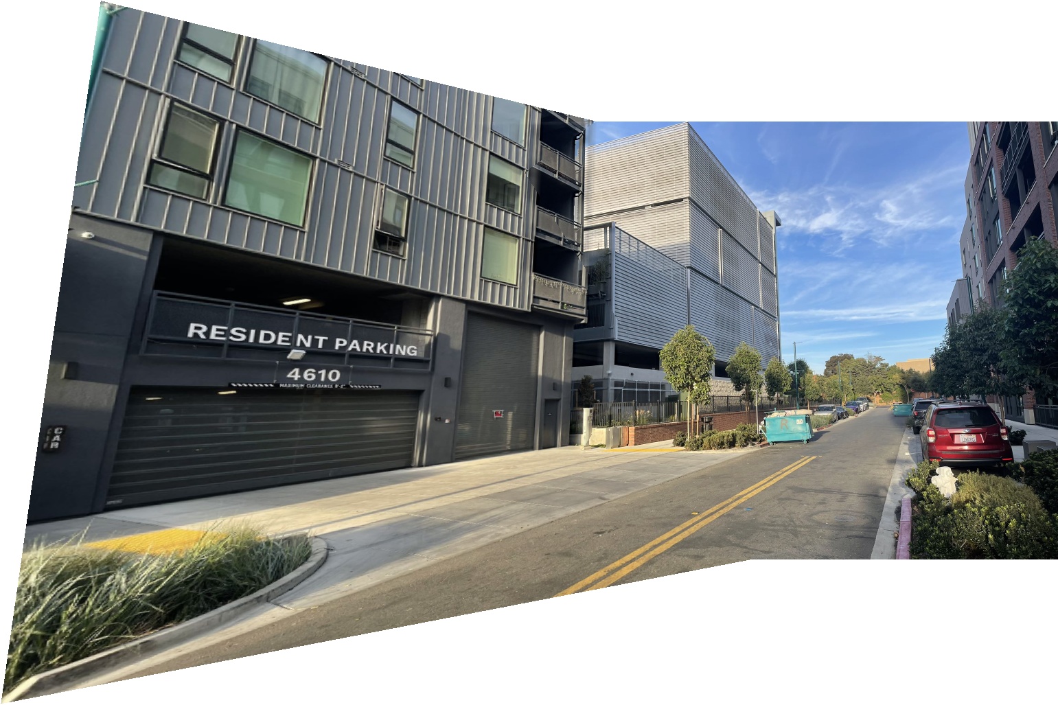
Final stitched garage image
Final Mosaic 1

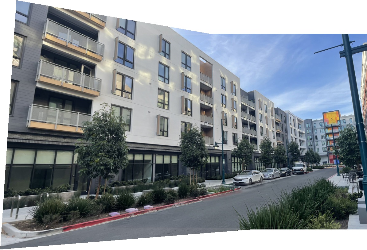
apartment left image

Final Mosaic 2

apartment right image

Stitched Balcony Image

Final stitched apartment image

Section 2: Automatic Stitching

Now that we have a way to stitch images together, it is natural to explore ways to automatically do this task. In this section, I will explore and create a system for automatically stiching images into a mosaic. I will present the system and algorithm step by step, and for most of the steps, I will be following the methods described in "Multi-Image Matching using Multi-Scale Oriented Patches" by Brown et al.

Step 1: Detecting Corner Features

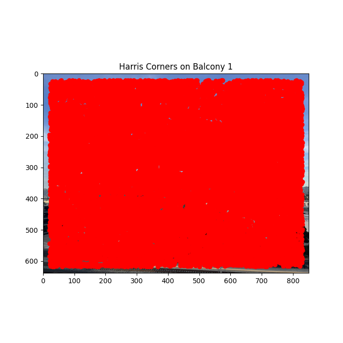
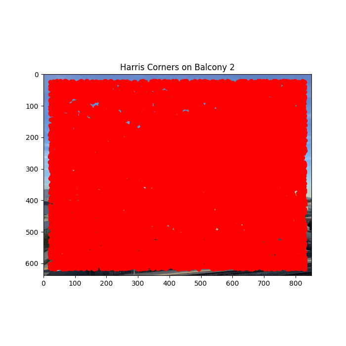
The first step is to find the interest points. To do this, I used a Harris corner detector to find the Harris corners in the image. What this is basically doing is using the gradients and the second moment matrix to identify the "corners" in the image (place where siginificant change in all directions occur). Below is an example of detected Harris corners on the two balcony images. As we can see, simply calculating the Harris corners give us very dense points, which makes it highly inefficient to help us match features in later steps.

Blend Image 1

Harris corners on balcony left image
Blend Image 2

Harris corner on balcony right image
Step 2: Adaptive Non-Maximal Suppression (ANMS)

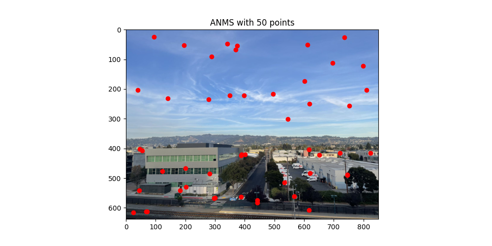
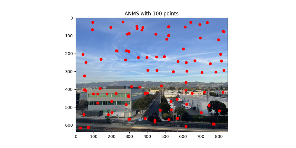
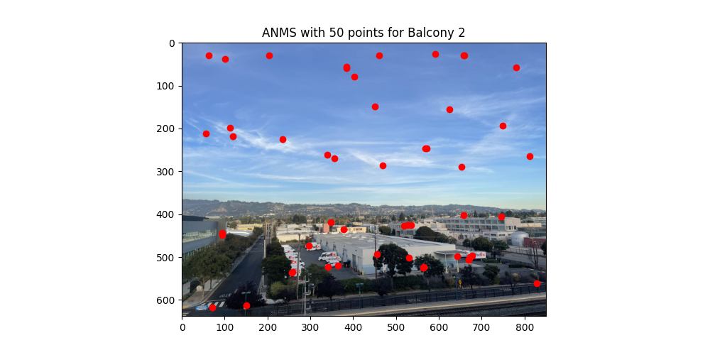
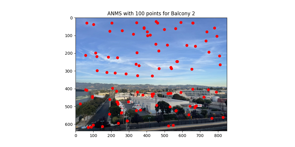
Once we have the Harris corners, we need to find a way to select a smaller subset of all the interest points. A smaller (and better) subset of interest point will improve the efficiency and accuracy for our algorithm. We want our points to 1. have large corner response, 2. evenly distributed in the image (not too clustered). In order to to this, we can use ANMS. The basic idea of ANMS is that each point is assigned a radius, defined to be the distance to the nearest stronger feature point. Mathematically, this is defined as \(r_i = \min_j |x_i - x_j|\) \(\forall x_j : h(x_i) < c_{robust} \cdot h(x_j)\), where \(r_i\) is the radius, \(x_i\) and \(x_j\) are feature point locations, \(h()\) is the corner response, and \(c_{robust}\) determines how much is "stronger" considered. Once we have all the radii, we can simply select the top K points with the largest radii. This will give us a very nice and evenly distributed set of interest points. Below is an example of applying ANMS with \(c_{robust} = 0.9\) on the balcony images for K = 100 and K = 50.
Blend Image 1
ANMS with K = 50 on balcony left image

Blend Image 2
ANMS with K = 100 on balcony left image

Blend Image 1

ANMS with K = 50 on balcony right image

Blend Image 2

ANMS with K = 100 on balcony right image

Step 3: Extracing Feature Descriptors

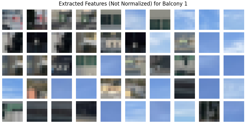
Now we have a good subset of the interest points, we need to extract feature descriptor using the interest points. To avoid aliasing,we first sample larger parches with radius 20 around the interest points (40*40 patches), we then sample with spacing s = 5 at a lower frequency than the one at which the interest points are located. For this part I used axis-aligned features and only one guassian level, and the features are also normalized afterwards. Below is an example of 50 features extracted from the balcony left image.

Blend Image 1

Feature extracted from balcony left image (Not normalized for better visualization)

Step 4: Feature Matching

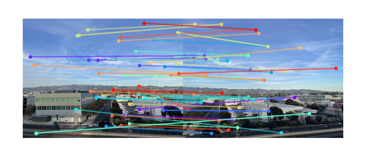
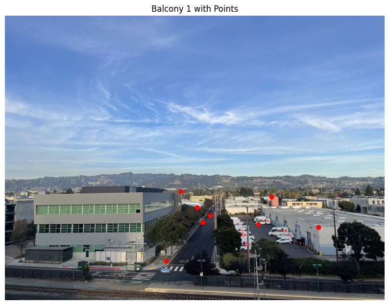
Now that we have the features, we need a way to match them. To do this, we can use nearest neighbor. First we calculate the distance between all pairs of features, then for each feature, we find its nearest neighbor and second nearest neighbor. We use the Lowe's trick (ratio between nearest and second nearest neighbor distance) to determine the best matches. The smaller the ratio is (nearest neighbor is much closer than the second nearest), the better the match is. Additionally, we can also filter out some outliers if the matching distance is larger than the average of second nearest neighbor distance from all points. Below is an example of feature matching performed on the balcony images.

Blend Image 1

Feature matching between balcony left and right images (corresponding points are connected)

Step 5: RANSAC

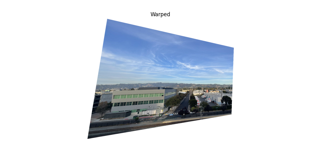
RANSAC stands for Random Sample Consensus. It is a robust way to estimate homography. RANSAC is used to further filter out outliers/inconsitency in the matches found in the previous step. To perform RANSAC, we randomly sample 4 pairs of points, calculate the exact homography transformation, and apply this transformation to every other pairs to see if they matches. We record the set of points which follows this computed homography (inliers), with a certain threshold. By repeating this process for a certain number of iterations, and keeping the largest set of inliers, we can use these inliers to estimate the homography transformation. RANSAC is very robust, as outliers that are different from the majority will be excluded. Below is an example of warping performed using the homography estimated by RANSAC.

Blend Image 1

original balcony left

Blend Image 2

balcony left warped with homography estimated by RANSAC

Automatic Stitching: Results

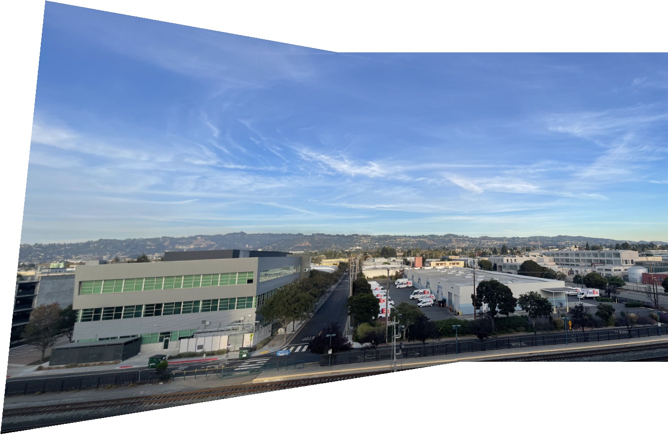
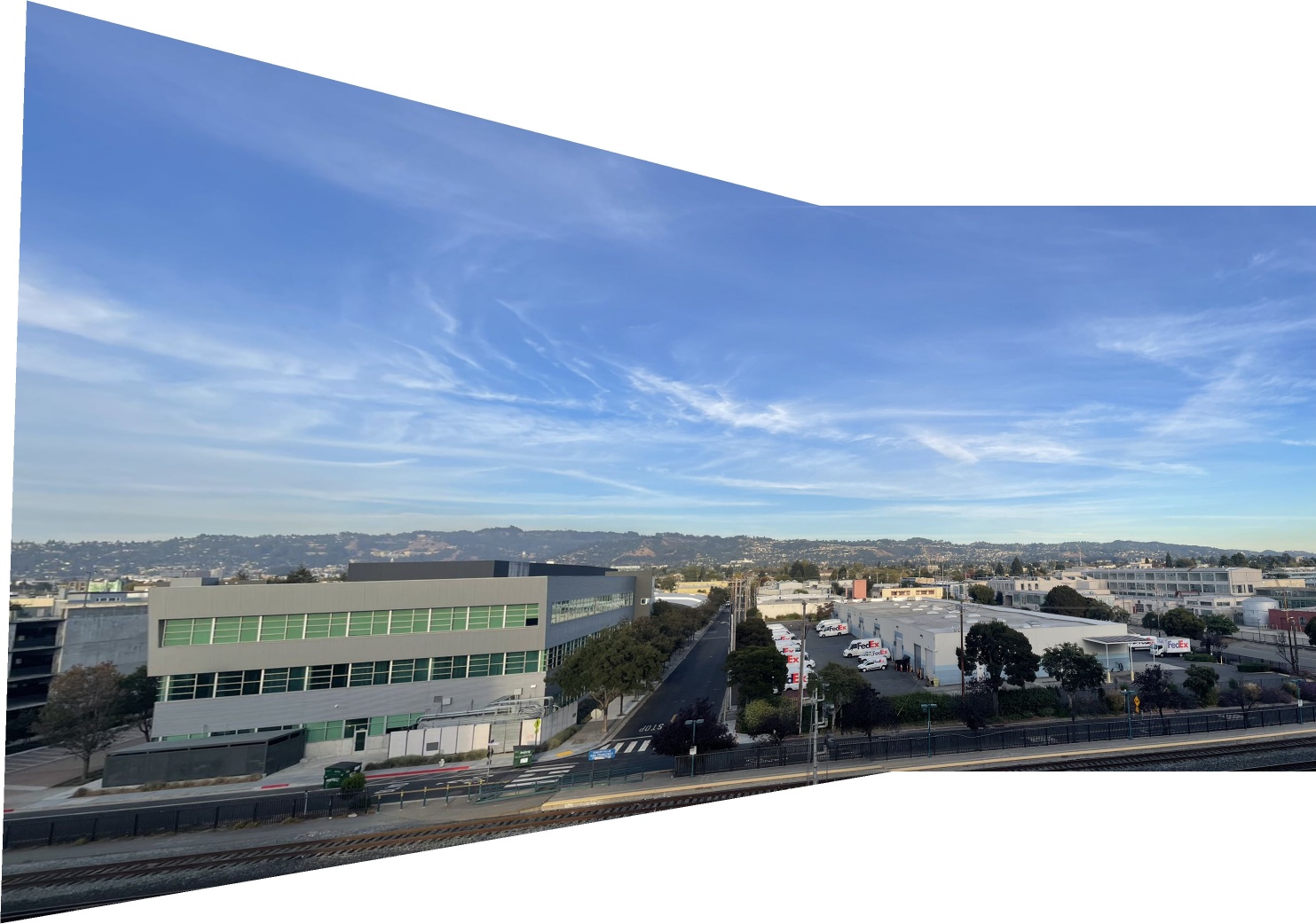
With all above steps, we are ready for automatic stiching. The actual stiching process is the same with manual stiching, except that the homography transformation is found automatically from the images instead of using manually labled points. Below are the comparisons between automatic stiching and manual stiching.

Blend Image 1

Automatic Stitched

Blend Image 2

Manually Stitched

Blend Image 1

Automatic Stitched

Blend Image 2

Manually Stitched

Blend Image 1

Automatic Stitched

Blend Image 2

Manually Stitched

Reflection

This was a very fun project and I enjoyed it a lot. The coolest thing I learned from this project is the power of majority. The application of RANSAC made me realize that majority is a very robust condition. Sometimes we don't need every data to be correct in order to make meaningful results, we only need the majority of the data to be correct. This also reminded me of the principle and assumption bitcoins relied on : the majority of computing power is owned by honest people. It is facsinating to see the robustness of majority.