Part A: Diffusion Models
Setup
In this project, we are using DeepFloyd IF diffusion model. This is a two stage model: the first stage produces images of size 64 x 64, and the second stage takes the output from the first stage and upscale it to 256 x256. Below are the results of generation using the three text prompts provided in the project spec. The quality of the image is quite nice, I am surprised they are quite good with only 20 denoising steps. Especially the picture of the man wearing a hat is very realistic. The images are also very related to prompt, as they reflect the prompt very well. The objects are exactly what being described in prompts, and also for first image, the image also accurately reflected the oil painting style mentioned in prompt. I am using the seed 1104.

an oil painting of a snowy mountain village (stage 1)

a man wearing a hat (stage 1)

a rocket ship (stage 1)
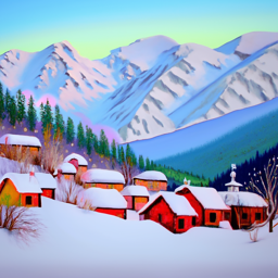
an oil painting of a snowy mountain village (stage 2)
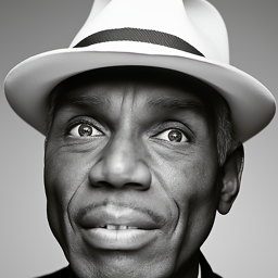
a man wearing a hat (stage 2)

a rocket ship (stage 2)
Noise Level Analysis
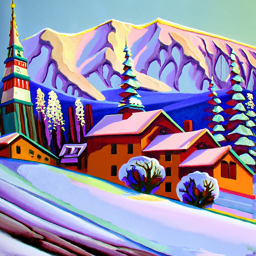
Below is the result of generation using the prompt "an oil painting of a snowy mountain village" using different number of denoising steps. We can see that with the increase of denoising steps, the image seems to be more colorful and detailed. Maybe more denoising steps allow the model to generate more "oil paintingness" in the image.
20 denoising steps
60 denoising steps
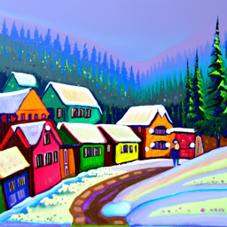
80 denoising steps
1.1 Implementing the Forward Process
For this part, I implemented the forward function. I got alpha_cumprod by indexing the t-th element in alphas_cumprod, and epislon is generated using torch.randn_like. Below are the Berkeley campinile at different noise levels.

Berkeley Campanile

Noisy Campanile at t=250

Noisy Campanile at t=500

Noisy Campanile at t=750
1.2 Classical Denoising
In this part I applied guassian bluring with kernel size equals 5 and sigma equals 3. Below are the side by side result of guassian blur filtering and the original noisy image.
Noisy Campanile at t=250
Noisy Campanile at t=500
Noisy Campanile at t=750

Gaussian Blur Denoising at t = 250

Gaussian Blur Denoising at t = 500

Gaussian Blur Denoising at t = 750
1.3 One-Step Denoising
To perform one-step denoising, I first use the forward process to generate a noisy image at given noise level t, then I use the stage 1 unet to predict the noise. Once I have the predicted noise, I obtained the clean image by solving for X0 in the equation \[ x_t = \sqrt{\bar{\alpha}_t}x_0 + \sqrt{1-\bar{\alpha}_t}\epsilon \quad \text{where} \quad \epsilon \sim \mathcal{N}(0,1) \] Below are the original image, and the noisy images and one-step denoised images at different noise levels.
Original Image
Noisy Campanile at t=250
Noisy Campanile at t=500
Noisy Campanile at t=750

One-Step Denoised Campanile at t = 250

One-Step Denoised Campanile at t = 500

One-Step Denoised Campanile at t = 750
1.4 Iterative Denoising
Creating a list of monotonically decreasing timesteps starting at 990, with a stride of 30, ending at 0, I followed this formula to iteratively denoise the image: \[ x_{t'} = \frac{\sqrt{\bar{\alpha}_{t'}}\beta_t}{1-\bar{\alpha}_t}x_0 + \frac{\sqrt{\alpha_t}(1-\bar{\alpha}_{t'})}{1-\bar{\alpha}_t}x_t + v_\sigma \] Below is a series of images during every 5th loop of denoising process. Further below, I have showed the original image, the iteratively denoised image, one-step denoised image, and gaussian blurred image for comparison.

Noisy Campanile at t=90

Noisy Campanile at t=240

Noisy Campanile at t=390

Noisy Campanile at t=540

Noisy Campanile at t=690
We can see that iteratively denoised image has the best quality, followed by one-step denoised image, and then gaussian blurred image has the worst quality.
Original

Iteratively Denoised Campanile

One-Step Denoised Campanile

Gaussian Blurred Campanile
1.5 Diffusion Model Sampling
In this part, I used iterative_denoise and set i_start = 0; I passed in random noise generated using torch.randn, and used the prompt embedding of "a high quality photo". Here are five results sampled using this procesure, with a seed of 1104.

Sample 1

Sample 2

Sample 3

Sample 4

Sample 5
1.6 Classifier-Free Guidance
Some of the images in the prior section are not very good. To address this, we can perform classifier-free guidance. This is done by computing both a noise estimate conditioned on the prompt, and an unconditional noise estimate, then we calculate our new noise estimate as: \[\varepsilon = \varepsilon_u + \gamma(\varepsilon_c - \varepsilon_u)\] where epsilon_u is the unconditional noise estimate, and epsilon_c is the conditional noise estimate, and gamma is the guidance scale. To get the unconditional noise estimate, we can simpy pass an empty prompt embedding to the model. The rest of the process is same as last part. Below are some results using classifier-free guidance and a seed of 2002.

Sample 1

Sample 2

Sample 3

Sample 4

Sample 5
1.7 Image-to-image Translation
If we take an image, add some noise to it, and then denoise it, we would get an image that is similar to the original image. The more noise we add and remove, the more different the denoised image would be from the original image. In this part, I added different amounts of noises to images, and then denoise them using text prompt "a high quality photo" to get new images (follows the SDEdit algorithm). Below are some examples with different noise levels.

SDEdit with i_start = 1

SDEdit with i_start = 3

SDEdit with i_start = 5

SDEdit with i_start = 7

SDEdit with i_start = 10

SDEdit with i_start = 20
Campanile

SDEdit with i_start = 1

SDEdit with i_start = 3

SDEdit with i_start = 5

SDEdit with i_start = 7

SDEdit with i_start = 10

SDEdit with i_start = 20

A Tree

SDEdit with i_start = 1

SDEdit with i_start = 3

SDEdit with i_start = 5

SDEdit with i_start = 7

SDEdit with i_start = 10

SDEdit with i_start = 20

A Car
1.7.1 Editing Hand-Drawn and Web Images
We can also apply SDEdit to hand-drawn and web images to force them onto the image manifold. Below are the results of applying SDEdit with different noise levels to web and hand-drawn images. The first one is a web image, and the second and last one are my hand-drawn images.

Volcano with i_start = 1

Volcano with i_start = 3

Volcano with i_start = 5

Volcano with i_start = 7

Volcano with i_start = 10

Volcano with i_start = 20

Volcano

Apple with i_start = 1

Apple with i_start = 3

Apple with i_start = 5

Apple with i_start = 7

Apple with i_start = 10

Apple with i_start = 20

Original Apple Sketch

SDEdit with i_start = 1

SDEdit with i_start = 3

SDEdit with i_start = 5

SDEdit with i_start = 7

SDEdit with i_start = 10

SDEdit with i_start = 20

Original Pumpkin Sketch
1.7.2 Inpainting
To do image inpainting, I first generate mask specifying the region I want to replace, then I run the diffusion denoising loop, but at every step, after obtaining x_t, I "force" x_t to have the same pixels as the original image where mask is 0, i.e: \[x_t \leftarrow \mathbf{m}x_t + (1-\mathbf{m})\text{forward}(x_{orig}, t)\] In this case, we only generate a new image inside the region we want to replace. Below are the results of inpainting for the Campanile and two of my own chosen images.
Campanile

Mask

Hole to Fill
.png)
Campanile Inpainted

Picture of People

Mask

Hole to Fill

People Inpainted

Neymar

Mask

Hole to Fill
.png)
Neymar Inpainted
1.7.3 Text-Conditional Image-to-image Translation
Now we will do SDEdit but guide the projection with a text prompt. The following results are SDEdit on different noise levels, with text prompt "a rocket ship". The first one is the campanile, and the last two are images of my own choices (also conditioned on "a rocket ship")

Rocket Ship at noise level 1

Rocket Ship at noise level 3

Rocket Ship at noise level 5

Rocket Ship at noise level 7

Rocket Ship at noise level 10

Rocket Ship at noise level 20
Campanile

Rocket Ship at noise level 1

Rocket Ship at noise level 3

Rocket Ship at noise level 5

Rocket Ship at noise level 7

Rocket Ship at noise level 10

Rocket Ship at noise level 20

Toothpaste

Rocket Ship at noise level 1

Rocket Ship at noise level 3

Rocket Ship at noise level 5

Rocket Ship at noise level 7

Rocket Ship at noise level 10

Rocket Ship at noise level 20

Ironman/p>
1.8 Visual Anagrams
To create a visual anagram that look like one thing normally but look like another thing upside down, we can denoise an image normally with one prompt, to get one noise estimate, we can then flipp it upside down and denoise with another prompt to get another noise estimate. We then flip the second noise esitame, and average the two. We then proceed with the denoising using the new averaged noise estimate. Below are some of the results, where the first image is the original image, and the second image is flipped upside down.
.png)
An oil painting of an old man

An oil painting of people around campfire

A parrot sitting on a tree branch

A blooming garden with flowers and trees
.png)
A lion under a tree
.png)
A person walking in the forest
1.9 Hybrid Images
To implement the make hybrids function, I will first estimate the noise separately using two different prompts, then create a composite noise estimate by combining the low frequencies from one noise stimate with high frequencies from the other, i.e.:
.png)
Hybrid image of a skull and a waterfall

Hybrid image of a lion and a skull
.png)
Hybrid image of flower patterns and a human skeleton